Excel: Data Entry and Formatting for Text and Numbers

By La Formula Magica Tech - Gianluca Bonomo

When working in Excel, one of the basics to really understand is this: Excel tries to automatically interpret what we write. And from there, it decides how to display it.

Text, for example, is normally aligned to the left. A number, on the other hand, is aligned to the right. It is a simple detail, but it already says a lot about how Excel is reading the contents of the cell.

If you learn to control this interpretation, you work better, make fewer mistakes, and get tidier and more professional sheets. The point is not just entering data. The point is to make them readable for Excel and also for those who will use the file.

🧭 How Excel recognizes what you write

When you enter a value in a cell, Excel immediately tries to understand what type of data it is.

• If you write a word or phrase, it considers it text.
• If you write a figure, it considers it a number.
• If you write something like 5%, it interprets it as a percentage.
• If you write a form like 2/5, it very often reads it as a date and not as a fraction.

And that is exactly where the interesting cases begin. Because Excel is often convenient, but sometimes it decides for us. And what it understands does not always coincide with what we had in mind.

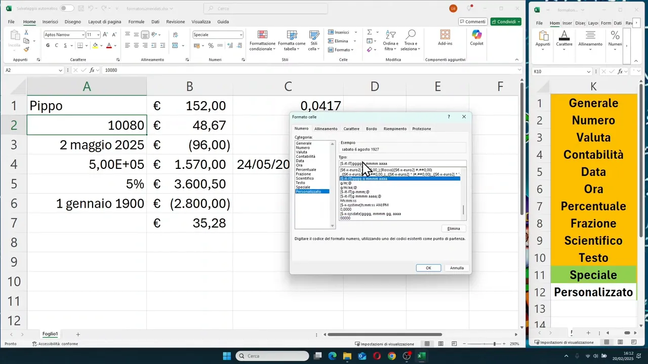
To verify the format associated with a cell, you can open the Format Cells window. The fastest method is Ctrl + 1. Alternatively, you can access it from the menu or by right-clicking with the mouse.

In the window, you will find the category assigned to the selected content. Many newly filled cells result in General, which is Excel's default format.

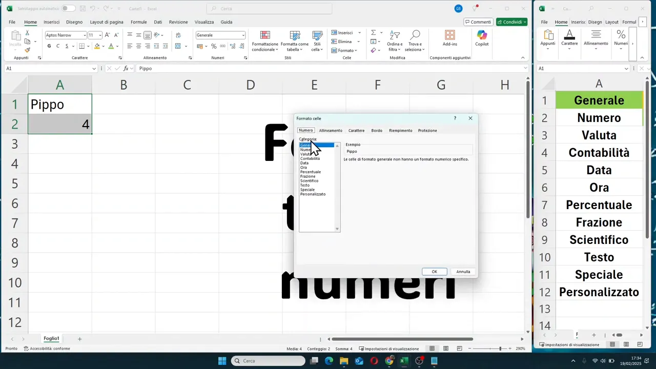
🔢 The General format and the Number format

The General format is what Excel applies when we don't tell it anything specific. It's fine for initial data entry, but has few controls.

If, on the other hand, you want to manage numbers better, it is best to use the Number format. Here you can decide:

• how many decimal places to show
• whether to use the thousands separator
• how to display negative numbers

For example, a value with many decimal places can be shown with two decimals, and thus rounded only in the display. Integers can become values with .00 if you want to standardize the column appearance.

You also have quick buttons in the toolbar to increase or decrease decimals. They are handy when you want to make a quick correction without reopening the Format Cells window every time.

For negative numbers, you can choose different views:

• with the minus sign
• in red
• in parentheses
• in red and in parentheses, in some cases

This aspect is particularly useful in accounting sheets, budgets, reports, and economic analyses.

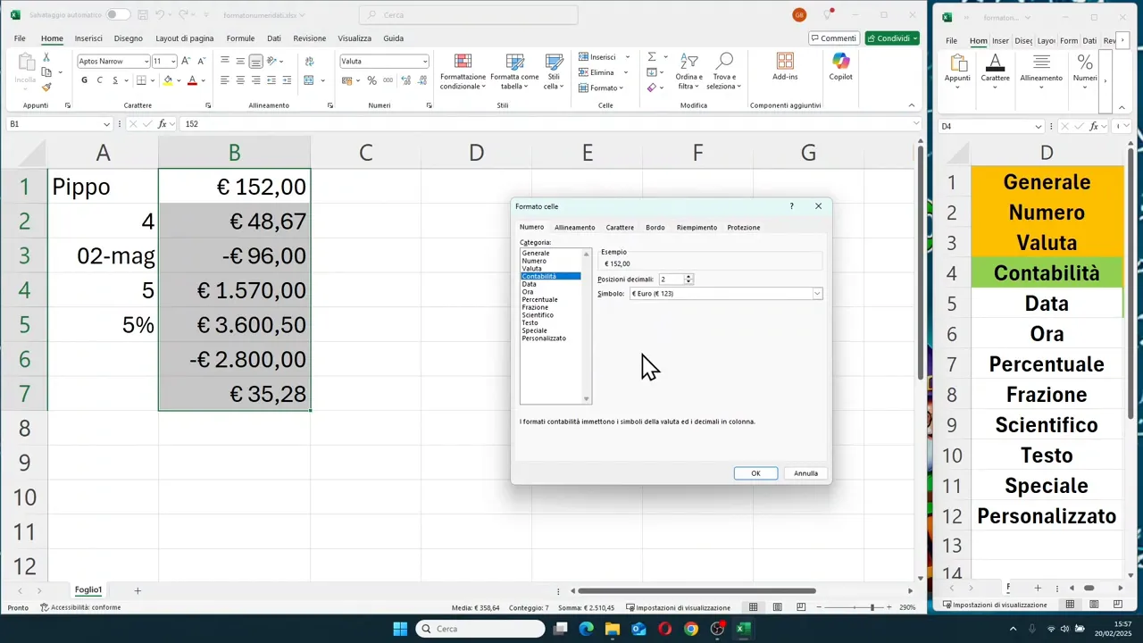
💶 Currency and accounting, they seem similar but are not the same

One of the most common mistakes is thinking that Currency and Accounting are the same thing. In reality, they have a very different logic in presentation.

Currency Format

With the currency format, you can add a monetary symbol to the number. It can be Euro, Dollar, Yen, and so on. You can also set:

• the number of decimal places
• the symbol position based on the chosen format
• the appearance of negative values

The symbol is shown next to the number, in a rather compact way.

In the case of the Euro, you can even choose a variant that shows it before the number or one that shows it after.

Accounting Format

The accounting format is designed for tidier and more readable tables. Here, the currency symbol is separated and aligned on the left side of the cell, while the number remains aligned to the right.

The result is a cleaner column, especially when comparing many amounts.

Another important difference is this: negative numbers are often shown in parentheses, without the minus sign in front. This is a typical convention in accounting statements.

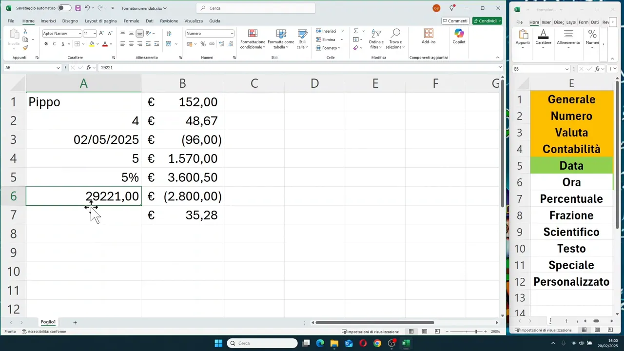
📅 The Date format and why Excel treats it as a number

The date is one of the most important points to understand. In Excel, a date is not just a readable text. Underneath, it is a number.

This explains many things:

• why you can add or subtract days
• why you can calculate differences between dates
• why a date can change its appearance without changing its actual value

If you enter a date like 2/5, Excel may interpret it as May 2nd. Then, through Format Cells, you can decide how to display it:

• numerical day and month
• month written in letters
• two-digit year
• four-digit year
• longer or more compact formats

The content remains the same. Only the display changes.

The most interesting part is that if you convert a date into a number format, Excel shows you its serial value. In practice, it counts the days starting from a base date in its system, which corresponds to January 1st, 1900.

So a date like May 2nd, 2025 corresponds to a very precise internal number. This number is not an error. It is exactly how Excel stores the date.

⏰ The Time format and its link to decimal numbers

Time, too, like the date, is linked to a number. Except in this case, we are talking about fractions of a day.

For example:

• 0.5 represents half a day, so 12:00 PM
• 1 represents a full day
• 0.1 corresponds to a part of the day, thus to a specific time

This means that Excel stores the time as a decimal value between 0 and 1, when referring to a single day.

If you write a time in the classic way, for example 13:01, Excel still converts it to its corresponding internal numerical value. It shows you the time, but in memory it is working with a number.

In the time format, you can choose whether to display:

• the 24-hour system
• the 12-hour system with AM and PM

And you can also combine date and time in the same cell. For example, by entering the date first and then the time, Excel can store both pieces of information together and display them in a single value.

📈 Percentages, the trick is to understand the underlying number

With percentages, a very simple rule applies. If you type 5% directly, Excel automatically recognizes it as a percentage.

If, on the other hand, you write 0.5 and then apply the percentage format, Excel will display it as 50%.

So the percentage format does not only change the appearance. It changes how the value is read on the sheet, starting from the fact that the percentage is linked to a decimal number.

Here too, you can decide the number of decimal places to display.

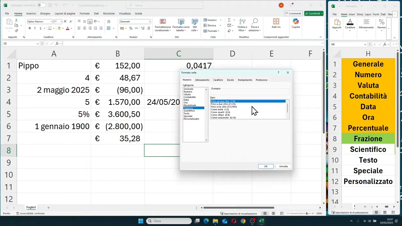
🍰 How to enter a fraction without it becoming a date

This is a classic case. You type 2/5 and Excel immediately thinks of a date. If, instead, you wanted a numerical fraction, you have to act beforehand.

The correct procedure is this:

1. select the cell
2. open Format Cells with Ctrl + 1
3. choose the Fraction category
4. only then type the value, for example 2/5

This way, Excel keeps it as a fractional number.

If, on the other hand, you have already typed 2/5 and Excel converted it into a date, changing the format afterward will not automatically return the original fraction. You will get the number associated with the date, not the 2/5 you had in mind.

So here, the keyword is: set the format first.

🔬 The Scientific format

The scientific format is used to represent very large or very small numbers in a compact form.

In practice, Excel shows the number with an initial part and an exponential notation. For example, a value like 5000 can be displayed as 5.00 with exponent 3. An even larger number will follow the same logic.

It is a useful format when working with:

• technical data
• mathematical values
• scientific measurements
• very large numbers that would take up too much space

It is not the most common format in daily sheets, but it is good to know it exists and how to read it correctly.

📝 The Text format and when to use it

If you apply the Text format to a cell, Excel treats the content as a string and aligns it to the left.

This is very useful when the value looks numerical but should not be treated as a number.

Think of cases like:

• product codes
• identifiers
• serial numbers
• internal codes

In these cases, you are not interested in performing calculations. You want to preserve the value as a label.

It is also a useful step when you want to prevent Excel from automatically modifying the content or interpreting it in an undesired way.

📮 Special formats

Excel also provides some special formats, designed for specific data types. Among those shown are:

• ZIP code / postal code
• fiscal code / tax ID
• phone number
• social security number

These formats serve to display the content with a structure more consistent with the data type, without having to manually intervene every time.

For example, a ZIP code remains a code and is not treated as a simple number to calculate.

⚙️ Custom format

If the standard formats are not enough, there is the custom format. Here, you can define how Excel should display the contents of the cell.

It is a very broad and powerful section. Excel already proposes several ready-made models, but you can also write your own pattern manually.

A classic example concerns the date. If you use four characters for the year, Excel shows the full year. If you use two, it shows it abbreviated.

The custom format is useful when you have precise layout needs or company standards to respect. It is not necessary to know it all right away, but it is worth knowing it is there and that it allows much more advanced control.

🛠️ All the ways to open Format Cells

Since you will use this window often, it is useful to remember the three main ways to open it:

• Ctrl + 1, the fastest
• from the menu Format > Cells
• with right-click > Format Cells

Personally, the keyboard shortcut remains the most convenient. Once memorized, you do everything much faster.

✅ Why the right format really makes a difference

Formatting well is not an aesthetic detail. It serves three fundamental purposes:

• making Excel understand what type of data you are entering
• avoiding wrong interpretations
• making the sheet clearer and more professional

If a fraction becomes a date, if a code is treated as a number, if an amount is not readable at first glance, the problem is not just graphical. It is operational.

For this reason, it is worth becoming familiar with the main formats: Number, Currency, Accounting, Date, Time, Percentage, Fraction, Scientific, Text, Special, and Custom.

Once you understand how Excel thinks, everything else becomes simpler.

❓ FAQ