Practical Excel and Geometry: How to Calculate Perimeter and Area with Formulas on Multiple Sheets

By La Formula Magica Tech - Gianluca Bonomo

When you really learn how to use Excel, the most important step is not making prettier tables. It is understanding how to link values entered in cells to formulas that work on their own.

A great exercise is geometry, because it forces you to think in a simple and practical way: you enter a few values, type the right formula, and the result updates automatically every time you change the numbers.

Here we will build four different sheets, one for the rectangle, square, circle, and right triangle, to get familiar with formulas, cell references, exponents, the pi function, and the square root.

📐 The workflow: a sheet for each shape

The idea is very clear: instead of putting everything on the same sheet, it is better to create a separate tab for each geometric shape. This way, the file remains tidy and each formula is easier to read, check, and edit.

For each sheet, it is best to always use the same logic:

• First row with the labels of the data to be entered.
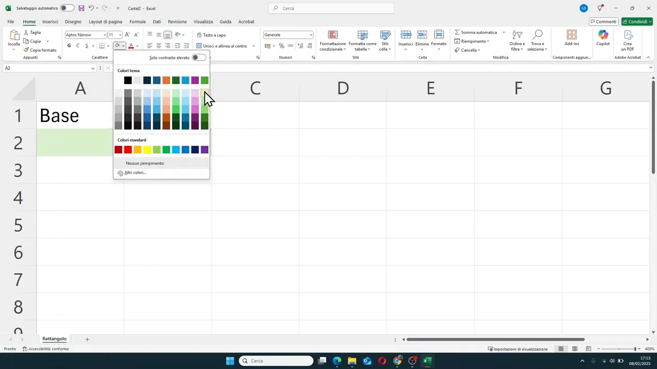
• Second row with the input cells, perhaps highlighted in green.
• Next row with the names of the results, such as perimeter, area, circumference, or hypotenuse.
• Results row with the formulas, highlighted in a different color.

This small visual trick immediately helps to distinguish where you write the numbers and where instead Excel needs to calculate.

🟩 How to set up the rectangle sheet

The first sheet can be renamed Rectangle. In the initial cells, you enter:

• A1: Base
• B1: Height
• A2 and B2: values to type
• A3: Perimeter
• B3: Area

Cells A2 and B2 are the reference cells. This means they will drive all calculations.

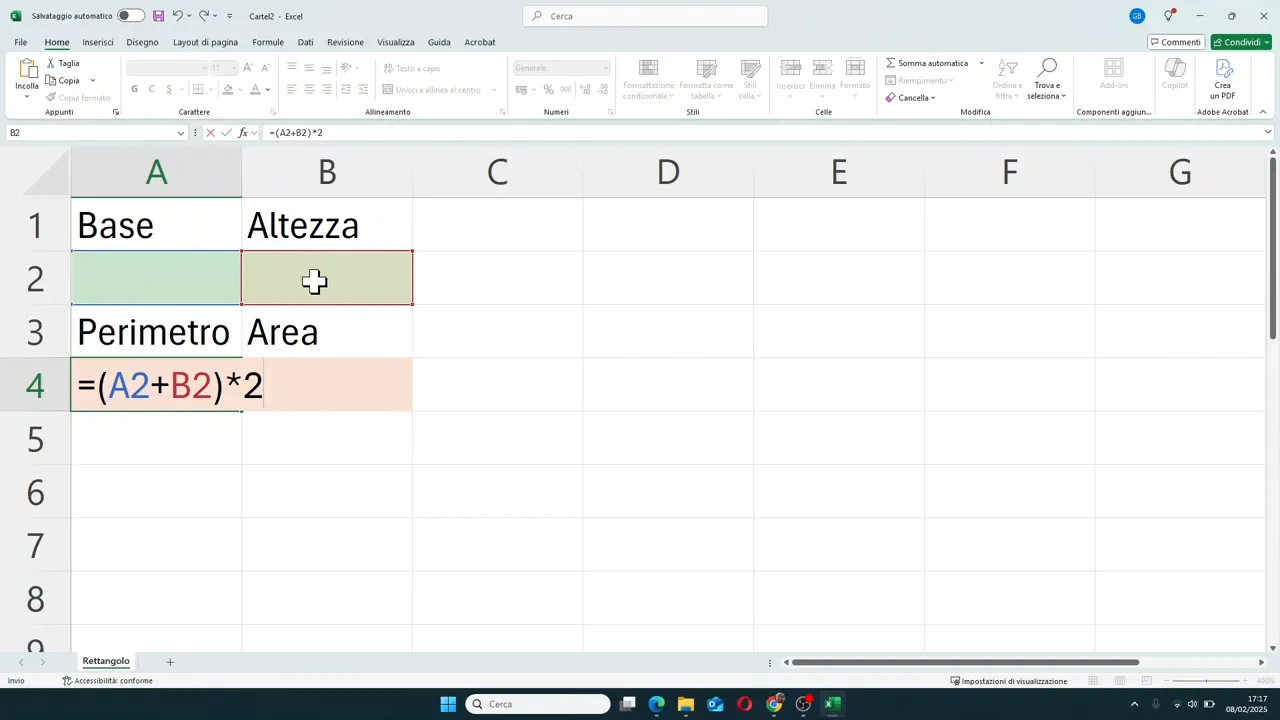
Formula for the perimeter of the rectangle

The perimeter of the rectangle is obtained by adding base and height, then multiplying the total by 2.

In Excel, the formula becomes:

= (A2+B2)*2

Parentheses are important because they force Excel to perform the addition first and then the multiplication.

Formula for the area of the rectangle

The area is even more direct: base times height.

=A2*B2

Once the formula is confirmed, the result will initially be zero if the input cells are empty. As soon as you enter the values, Excel automatically updates the result.

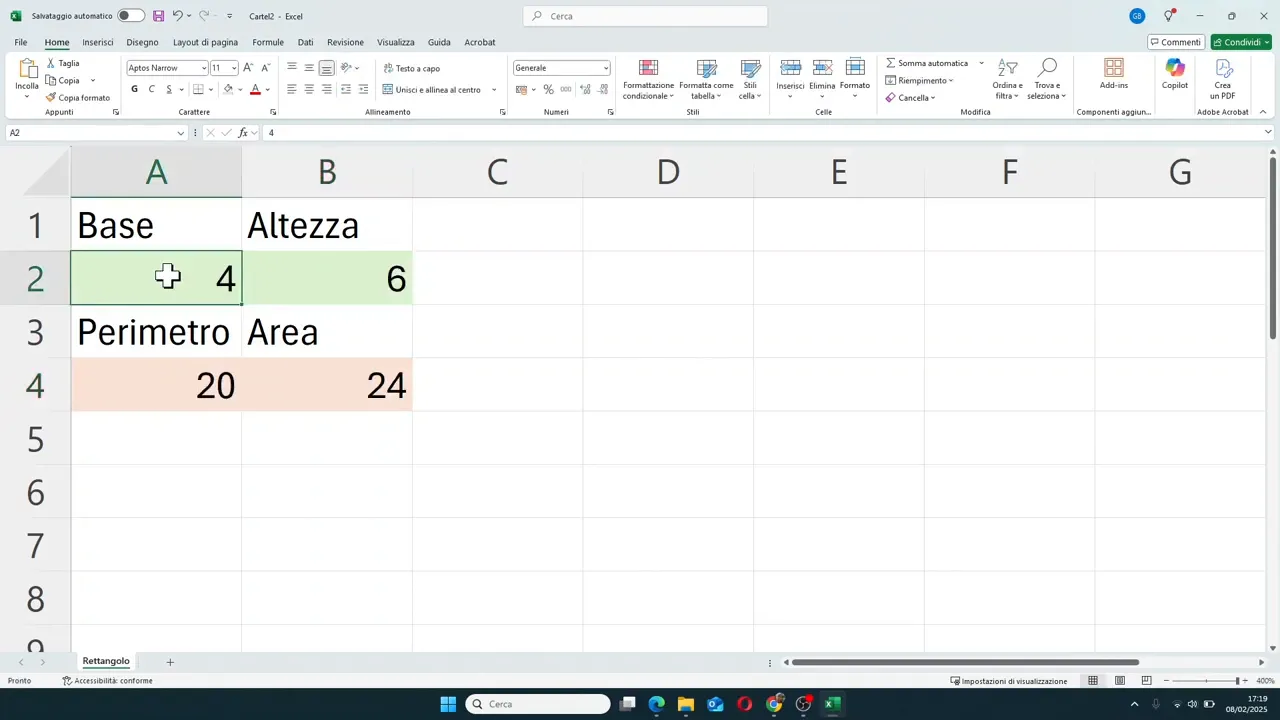
For example, with base 4 and height 6 you get:

• Perimeter: 20
• Area: 24

🟦 How to view and edit a formula in Excel

A very useful step, especially when you start, is learning to check what you wrote inside a cell.

You have three practical ways to do it:

• double-click on the cell containing the formula
• press F2 on the keyboard
• select the cell and look at the formula bar at the top

This is essential because it allows you not only to read the formula, but also to correct it on the fly if you made a mistake with a reference or an operator.

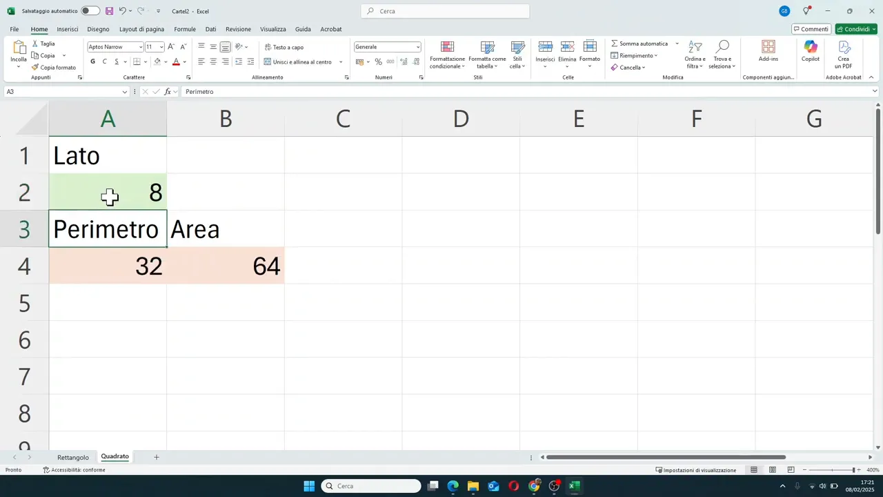
🟨 The square sheet

In the second sheet, to be renamed Square, only one starting piece of data is needed: the side.

• A1: Side
• A2: side value
• A3: Perimeter
• B3: Area

Formula for the perimeter of the square

The perimeter is the side multiplied by 4:

=A2*4

Formula for the area of the square

The area is the side squared. In Excel, exponentiation is written with the symbol ^.

=A2^2

This is a very important point: if you need to do an exponentiation, you do not write "squared" in words, but you use the correct mathematical symbol.

For example, if the side is 5:

• Perimeter: 20
• Area: 25

The interesting thing is that you only need to change the side value to immediately see everything else update. This is where you really see the convenience of formulas.

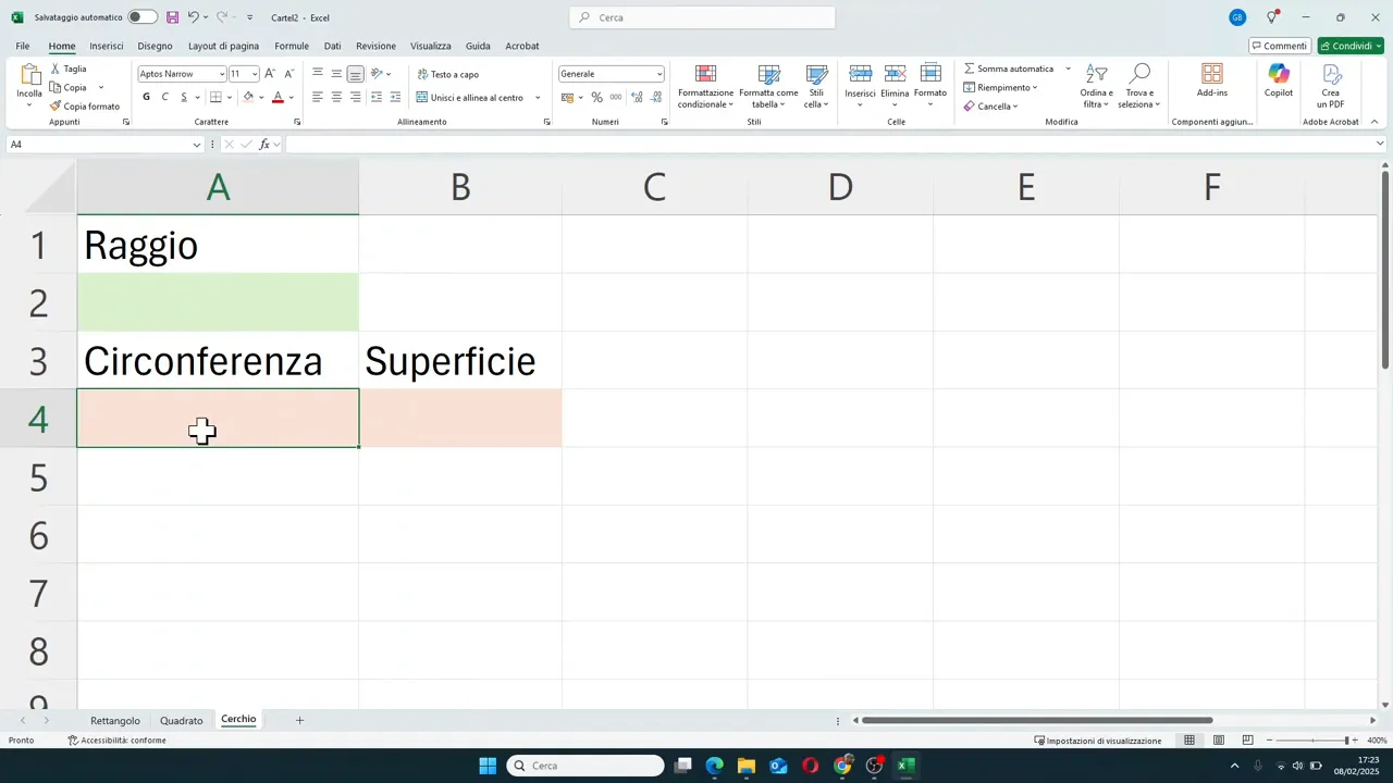
🔵 The circle sheet

Moving on to the circle, the starting value is the radius. The results to calculate are:

• circumference
• area

This part is very useful because it introduces a specific Excel function: the one that returns the value of pi.

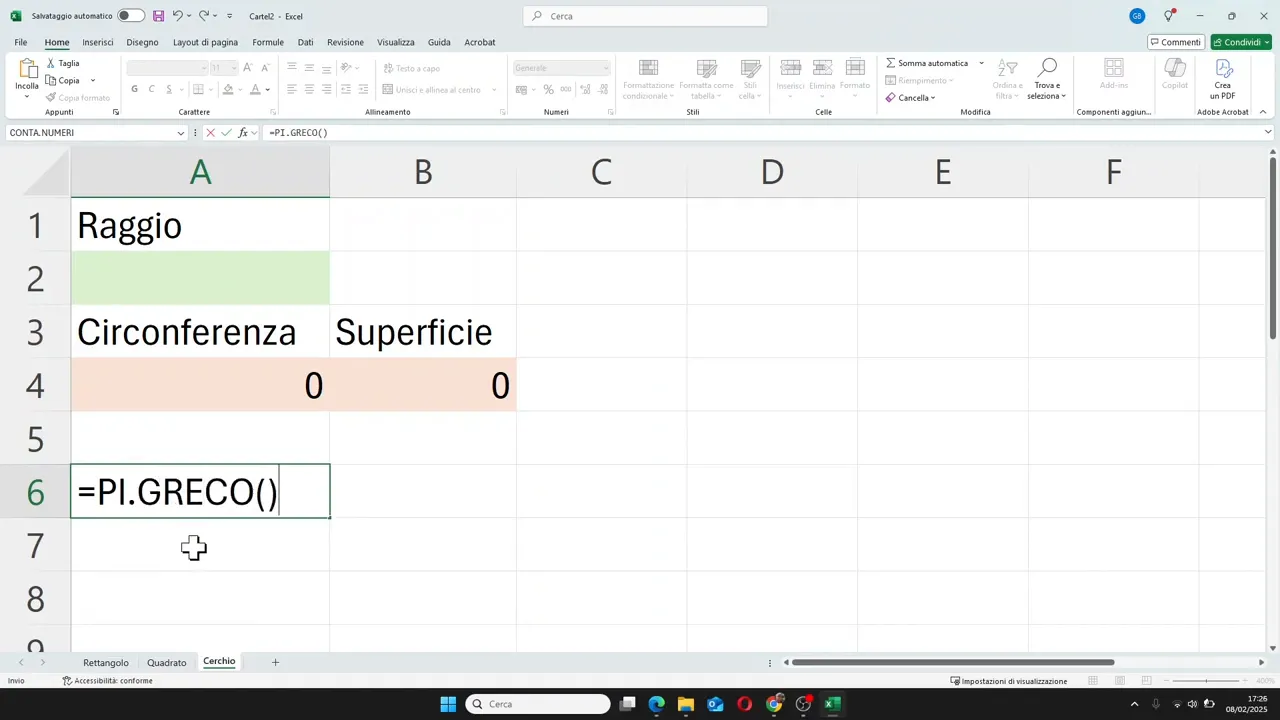
How to use pi in Excel

In Excel, pi is not written by hand as 3.14. A dedicated function is used:

=PI()

This function returns the value of pi with several decimal places. It is much better than entering it manually, as it makes the calculation more precise and professional.

Formula for the circumference

The circumference is calculated as 2 times pi times the radius.

=2*PI()*A2

Formula for the area of the circle

The area is calculated as pi times radius squared.

=PI()*A2^2

Here too, the exponentiation operator seen in the square comes in handy.

With radius 3, for example, you get approximately:

• Circumference: 18.85
• Area: 28.27

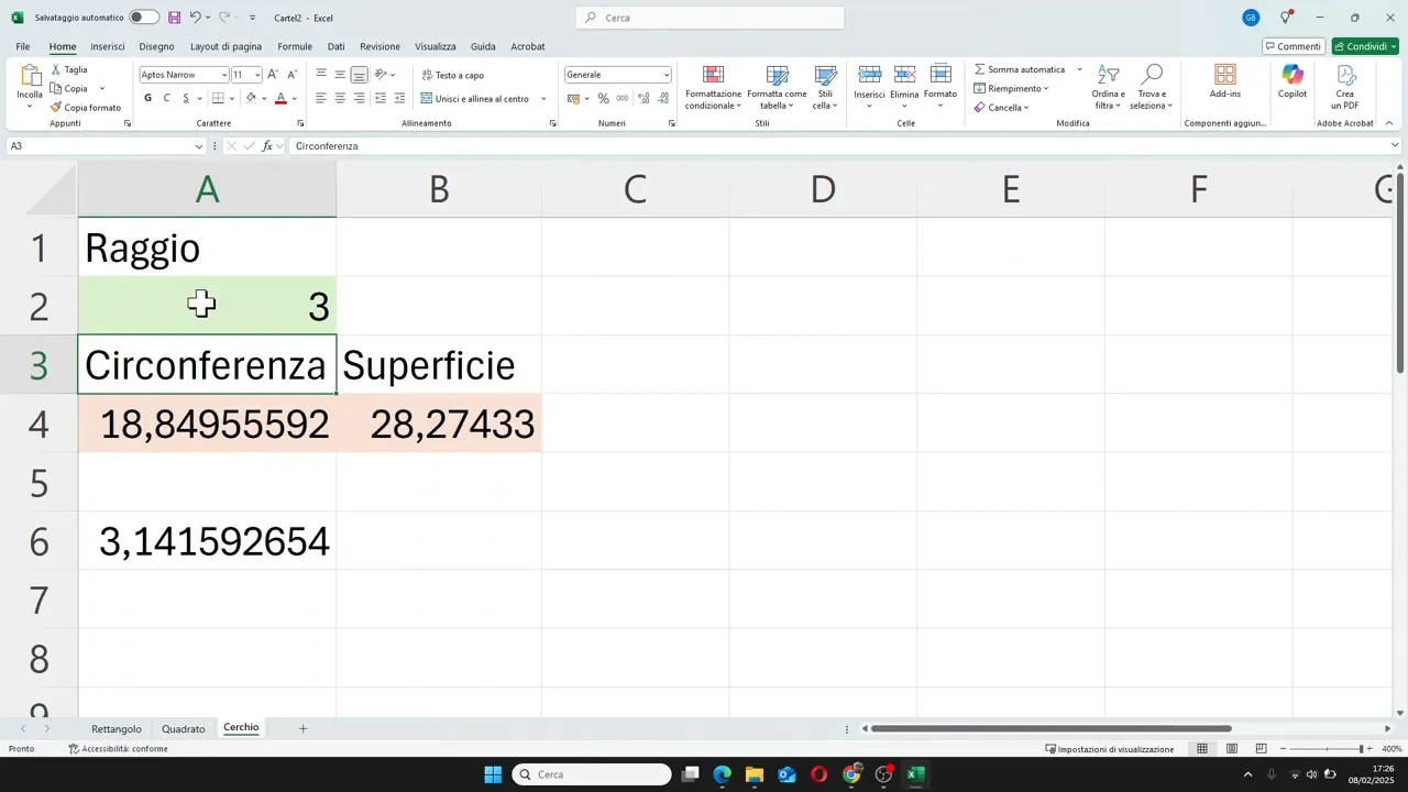
If you change the radius, the results update instantly in this case too.

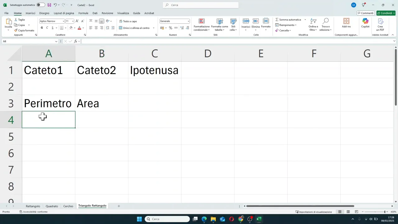
🔺 The right triangle sheet

The last example is also the most interesting, as it combines simple formulas and a compound formula.

In the Right Triangle sheet, the headers are:

• A1: Leg1
• B1: Leg2
• C1: Hypotenuse
• A3: Perimeter
• B3: Area

The two legs are values to be entered manually. The hypotenuse, however, is not typed: it is calculated.

Formula for the perimeter of the right triangle

The perimeter is simply the sum of the three sides:

=A2+B2+C2

But beware: this formula only works well if the hypotenuse cell already contains its correct calculation.

Formula for the area of the right triangle

In a right triangle, the area is obtained by multiplying leg by leg and dividing by 2.

=A2*B2/2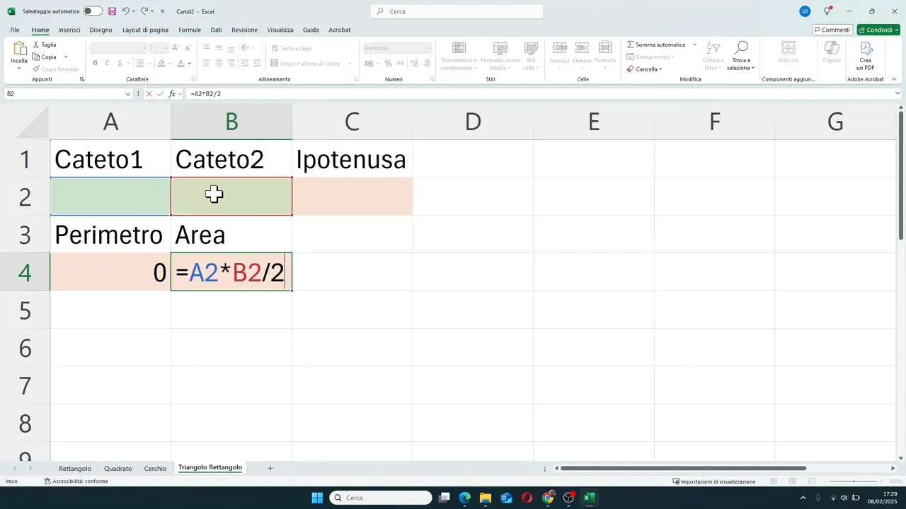

How to calculate the hypotenuse with the Pythagorean theorem

Here, the Pythagorean theorem comes into play. In practice:

• square the first leg
• square the second leg
• add the two results
• take the square root of the total

In Excel, the square root is obtained with the SQRT function.

=SQRT(A2^2+B2^2)

This formula goes into the hypotenuse cell.

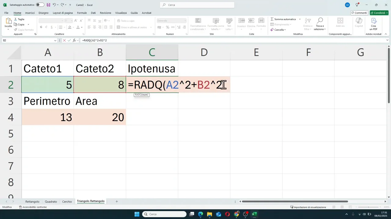
If you enter, for example, leg 1 as 5 and leg 2 as 8, Excel automatically calculates:

• Hypotenuse: approx. 9.43
• Perimeter: approx. 22.43
• Area: 20

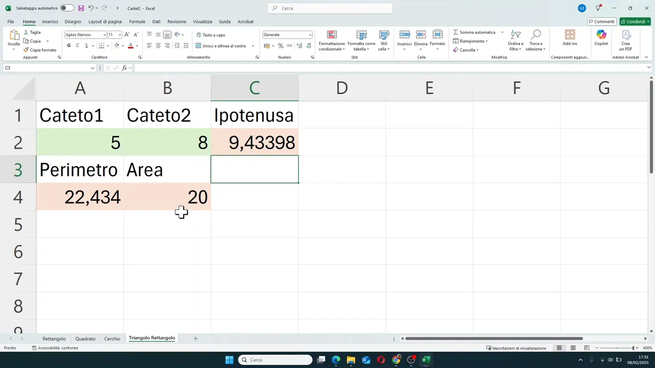
If you change one of the legs, not only the perimeter and area change automatically, but also the hypotenuse. This is an excellent example of a formula linked to other formulas.

🌐 When you don't know the formula, do this

A very practical idea to always keep in mind is this: you don't need to know everything by heart.

If you don't remember a geometric formula or the exact name of an Excel function, you can search for it and then apply it immediately in the worksheet.

The correct process is:

1. understand which quantity you want to calculate
2. find the correct mathematical formula
3. translate the formula into cell references
4. use Excel functions when needed, such as PI() or SQRT()

This approach applies not only to geometry, but to any use of Excel: mathematics, data analysis, quotes, reports, and business management.

⚙️ The most useful functions and operators used in these examples

To recap, here are the main tools used in the calculations:

• = to start a formula
• + to add
• * to multiply
• / to divide
• () to prioritize calculations
• ^ to raise to a power
• PI() for pi
• SQRT() for the square root

If you master these elements, you already have a very solid base to build many useful formulas in Excel.

🚀 Why this exercise is more useful than it seems

On the surface, it's just geometric shapes. In reality, you are training much broader skills:

• organizing data across multiple sheets
• using cell references correctly
• writing formulas without syntax errors
• distinguishing between inputs and outputs
• building models that update automatically

And that is exactly the leap in quality that makes Excel a truly useful tool in everyday work as well.

❓ FAQ