If you want to start using Excel in a truly useful way, there is a fundamental step to understand right away: formulas are not made by writing only fixed numbers, but by linking calculations to worksheet cells.
This is precisely what makes Excel powerful. You enter a formula only once, then when you change the values in the cells, the result updates itself. And this is where you start working more professionally.
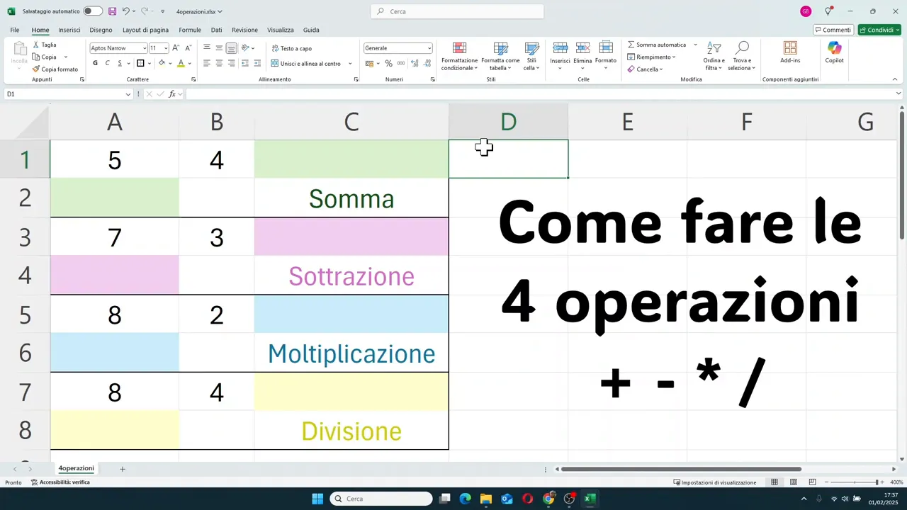
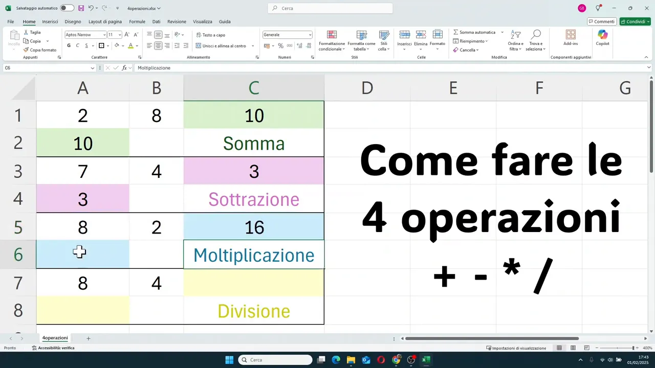
The first operations to learn are the four basics of mathematics:
- addition
- subtraction
- multiplication
- division
The logic is always the same: you write the equal symbol, indicate the cells involved, and insert the correct operator.
Table of contents
- 📘 Why use cell references
- 🧮 The structure of a formula in Excel
- ➕ How to sum with cell references
- 🔄 The real advantage: automatic update of results
- 👀 How to view or modify an already entered formula
- ➖ How to subtract
- ✖️ How to multiply
- ➗ How to divide
- 🛠️ Keyboard or mouse method: which is better?
- 🧠 The rule to always remember
- ❓ Frequently Asked Questions
- ✅ Conclusion
📘 Why use cell references
Imagine you have a number in A1 and another in B1. You could write a formula like 5+4, sure. But by doing so, you are locking the calculation to those two numbers.
If instead you write a formula that uses A1 and B1, Excel no longer computes based on handwritten numbers in the formula. It computes based on the content of the cells.
This means that if the value in A1 or B1 changes, the result changes automatically. This is the basic principle of almost everything you will do in Excel going forward.
🧮 The structure of a formula in Excel
Every formula always starts with a mandatory element: the equal sign.
This symbol serves to make Excel understand that inside that cell you are not writing simple text, but executing a calculation.
The simplest structure is this:
- equal sign
- first cell
- mathematical operation
- second cell
Example:
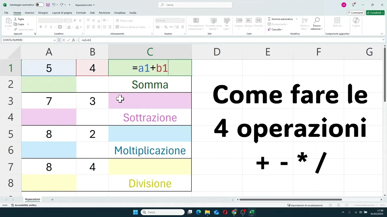
- =A1+B1
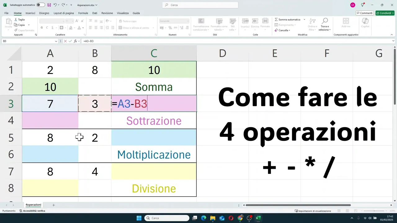
- =A3-B3
- =A5*B5
- =A7/B7
After writing the formula, simply press Enter to confirm.
➕ How to sum with cell references
Let's start with the most immediate operation. If you have a number in cell A1 and another in cell B1, you can get the sum in a third cell, for example, C1.
The procedure is this:
- click on the cell where you want the result
- write =
- insert A1
- write +
- insert B1
- press Enter
The result will appear immediately in the chosen cell.
If you prefer, you don't even have to type the references from the keyboard. You can do this:
- click on the result cell
- write the equal sign
- click with the mouse on the first cell
- write the plus sign
- click on the second cell
- press Enter
Excel inserts the names of the cells automatically as you select them.
The same sum can also be displayed in another cell, for example, A2, simply by repeating the same scheme. It doesn't matter where you put the result. It only matters that the formula points to the correct cells.
🔄 The real advantage: automatic update of results
Here you can truly see the strength of Excel.
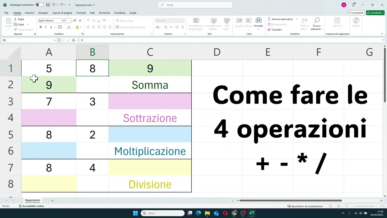
Let's assume that in the initial sum the values are 5 and 4. The result will be 9. If you then change the content of B1 and write 8 instead of 4, Excel immediately recalculates the result without you having to redo anything.
The same happens if you change A1. As soon as you confirm the new value with Enter, all cells depending on that reference update automatically.
In practice, the formula remains identical, but the result changes based on the data present in the linked cells.
This is the difference between using Excel like a simple calculator and using it as a true spreadsheet.
👀 How to view or modify an already entered formula
When there is a result in a cell, Excel shows the final number. However, the formula remains always available.
To check it, you have several ways:
- click once on the cell and look at the formula bar at the top
- double-click on the cell to enter edit mode directly
- press F2 on the selected cell to edit the formula via keyboard
This is very useful when you want to verify a calculation, correct a reference, or simply understand how a result was built.
➖ How to subtract
Subtraction follows exactly the same logic as addition. Only the operator changes, which in this case is the minus sign.
If you want to subtract the content of B3 from that of A3 and show the result in C3, you will write:
- =A3-B3
Press Enter and the result appears immediately.
The same calculation can be repeated in another cell, for example, A4, always pointing to the same references.
A useful detail: if you write the references in lowercase, Excel automatically capitalizes them. So a3-b3 is still interpreted correctly.
Here too, the same rule as before applies: if you modify the numbers in the starting cells, the result changes too.
✖️ How to multiply
To multiply two cells in Excel, you do not use x but the asterisk.
If you want to multiply A5 by B5, the formula will be:
- =A5*B5
After Enter, you get the product.
You can insert it in any cell you wish, for example, C5 or A6, as long as the reference points to the cells containing the values to be multiplied.
This is a point that often creates confusion at the beginning, so it's better to establish it clearly: to multiply in Excel, use *, not the letter x.
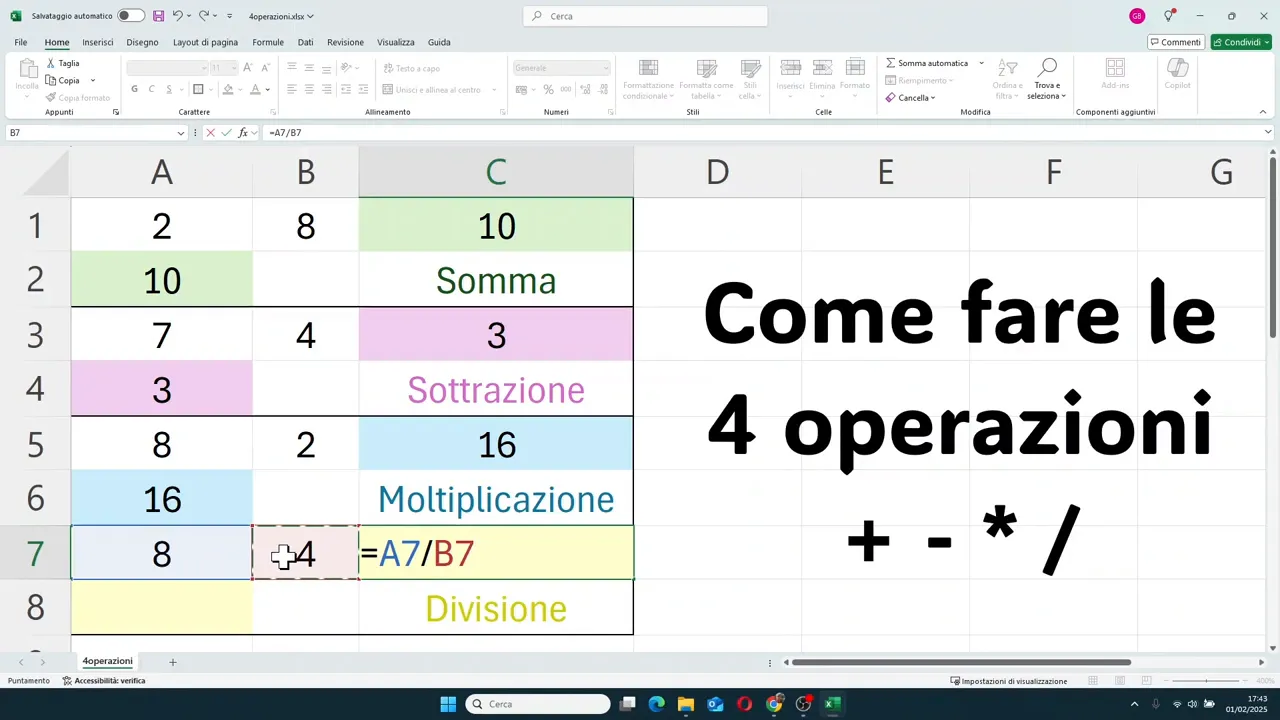
➗ How to divide
To divide, the correct operator is the forward slash.
If you have a value in A7 and one in B7, the formula to write will be:
- =A7/B7
Once confirmed with Enter, Excel returns the quotient.
In this case as well, the structure never changes:
- equal sign
- first cell
- operator
- second cell
🛠️ Keyboard or mouse method: which is better?
You have two main ways to build these formulas:
- writing references by hand, for example, =A1+B1
- clicking on the cells with the mouse while composing the formula
Both work well.
If you are at the beginning, clicking on the cells is convenient because it reduces errors and helps you get familiar with references. If instead you start working faster, writing from the keyboard can save you time.
The important thing is to understand the mechanism, because once you learn this, the rest of Excel formulas become much easier to tackle.
🧠 The rule to always remember
If I had to summarize everything in a single sentence, it would be this: in Excel, you start from the equal sign and then link the cells together with the necessary operation.
This applies to addition, subtraction, multiplication, and division.
So:
- for adding use +
- for subtracting use -
- for multiplying use *
- for dividing use /
And always remember that the result is dynamic, because it depends on the values present in the referenced cells.
❓ Frequently Asked Questions
Why must I start a formula in Excel with an equal sign?
Because the equal sign tells Excel that the content of the cell is a calculation. Without that symbol, the program interprets what you write as simple text.
How do you multiply in Excel?
You use the asterisk. For example, to multiply the contents of A5 and B5 you must write =A5*B5.
How do you divide in Excel?
You use the forward slash. A correct example is =A7/B7.
Is it better to write cell references or click them with the mouse?
Both methods are valid. If you are starting, clicking cells can help you avoid errors. When you gain more confidence, typing them directly can be faster.
How do I see the formula instead of the result?
You can click the cell and look at the formula bar at the top, double-click the cell, or press F2 to enter edit mode.
If I change a number in the starting cells, do I have to redo the formula?
No. If the formula uses cell references, Excel automatically updates the result as soon as you confirm the new value.
✅ Conclusion
Learning to create simple formulas with cell references is one of the first real steps to using Excel well.
You are not just doing calculations. You are building a sheet that reacts to data, updates automatically, and allows you to work in a much more orderly and reliable way.
Once you understand this mechanism, subsequent formulas will seem much less complicated. And it all starts here: =, cells, operator, Enter.