Excel from Zero to Wow: Create and Format Your First Table

By La Formula Magica Tech - Gianluca Bonomo

A well-made table instantly changes the look of an Excel file. Even with very simple data, it takes just a few steps to turn a blank sheet into something organized, readable, and professional.

The goal here is exactly this: to start from scratch and build a complete table, entering data, arranging columns, formatting numbers, adding borders, colors, and a minimum of graphic care. No unnecessary complications. Only the operations you really need to get a clean result.

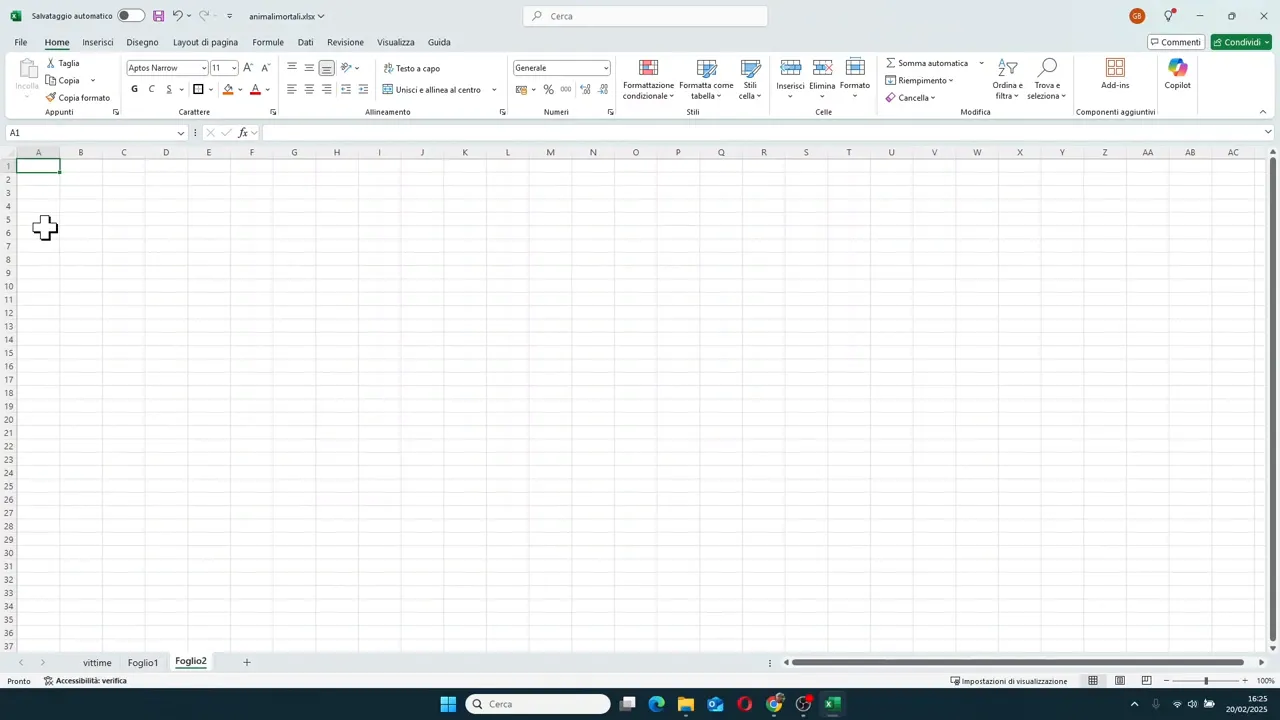
🧩 From a blank sheet to a clear structure

When you open Excel, you find yourself in front of the classic blank sheet. The first step is very simple: start typing the table headers.

In the example, a table with four columns is built:

• Rank
• Organism
• Annual victims
• Primary cause of death

You start from cell A1 and move to the right, one cell at a time. To do this, you can use the keyboard arrows or click directly with the mouse in the next cell.

An important thing: at the beginning, there is no need to waste time widening the columns. It is better to write everything first. If the text overflows into adjacent cells, it is not a problem. You will fix it later much faster.

⌨️ Entering data without complicating your life

After the headers, we move on to the actual data. In the example, several organisms are listed with their relative number of annual victims and the associated primary cause.

Here the key point is to work simply:

• type one value per cell
• move with the arrows or mouse
• continue row after row

For numbers, there is no need to type thousands separators or other symbols. Enter the number cleanly, for example 725000, and let Excel format it later.

This approach saves you time and reduces errors. Content is loaded first, then you work on the appearance.

📏 Widening columns automatically

Once the data is entered, one of the most useful steps of all arrives: adapting the column width to the content.

If you have long headers or longer texts, some columns will be too narrow. Instead of dragging them by hand one by one, you can use the fastest method:

1. select the columns involved, in the example from A to D
2. hover over the border between two column headers
3. double-click

Excel will automatically widen or narrow each column based on the longest content inside it.

It is a small trick, but it makes a big difference when you want to achieve order in seconds.

🎯 Centering and bolding headers

Headers guide the reading of the table. Because of this, they deserve to be highlighted a bit.

In the example file, the header cells are:

• horizontally aligned to the center
• set to bold

To center the text, simply select the four cells in the first row and use the center alignment command in the toolbar.

For bold, you can click on the dedicated icon or use the keyboard shortcut shown in the tutorial, which is Ctrl + B (or Ctrl + G in Italian Excel).

The result is immediate: the header row stands out better from the rest of the table and the content is more readable.

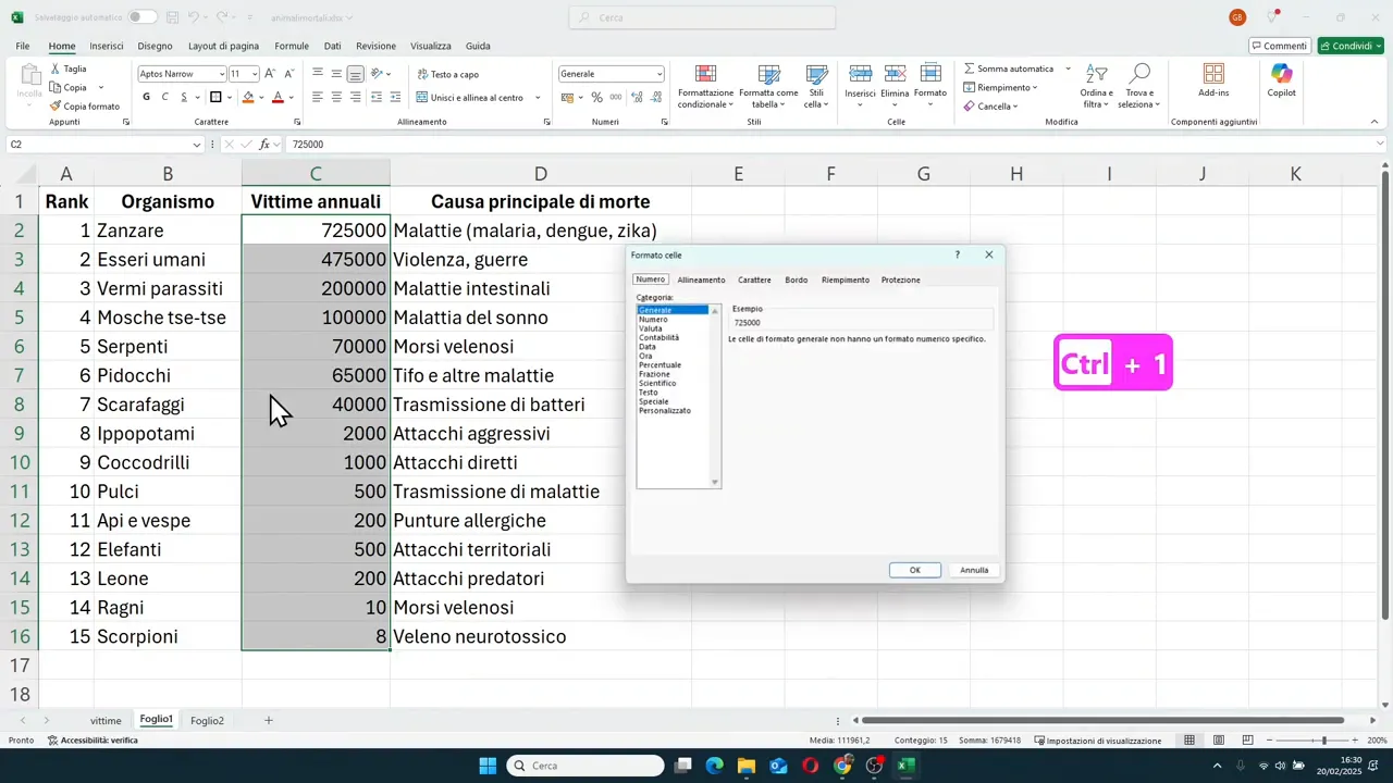
🔢 Formatting numbers with the thousands separator

Raw numerical values are correct, but often difficult to read. A number like 725000 is much clearer if it becomes 725,000.

To achieve this effect, you have two ways.

Method 1: Format Cells

1. select the cells with the numbers
2. press Ctrl + 1 to open the Format Cells window
3. choose the Number category
4. set decimal places to zero
5. activate the thousands separator

Method 2: Quick button in the toolbar

You can also use the comma style separator button. In this case, Excel applies the separator, but it may also add decimal places. If that happens, just use the decrease decimal command to reduce them to zero.

This step makes the numbers much more readable, especially when the values are large.

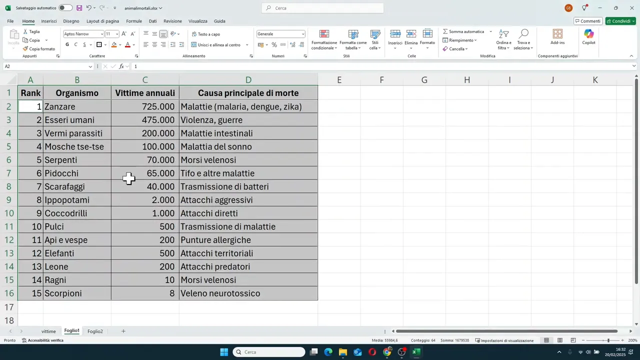
🧱 Using borders to give the table structure

A table without borders often looks flat or scattered. Borders help the eye follow rows and columns more easily.

In the example, a simple but effective combination is used:

• thin borders on all cells
• thick outside borders on the header and the entire table area

The process consists of first selecting the header and then, while holding down Ctrl, the data block below. At that point, apply all borders and then the thick outside border.

This way the table immediately gains a more defined and professional shape, without needing complicated effects.

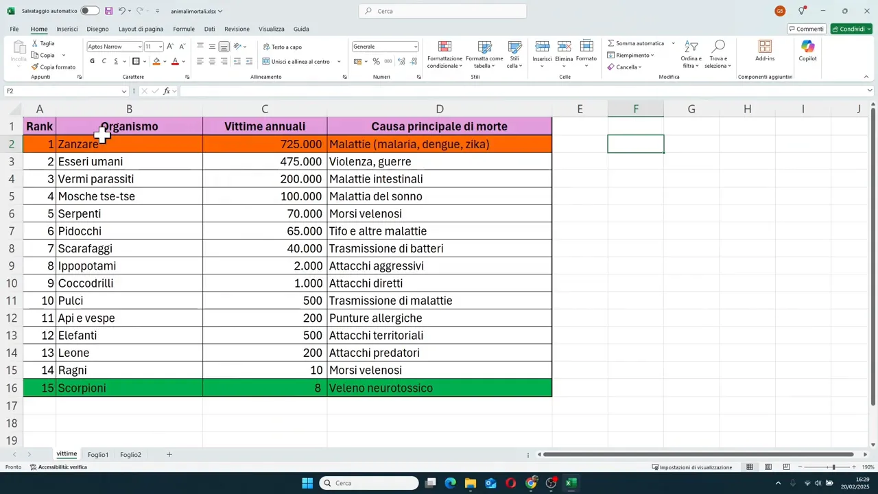
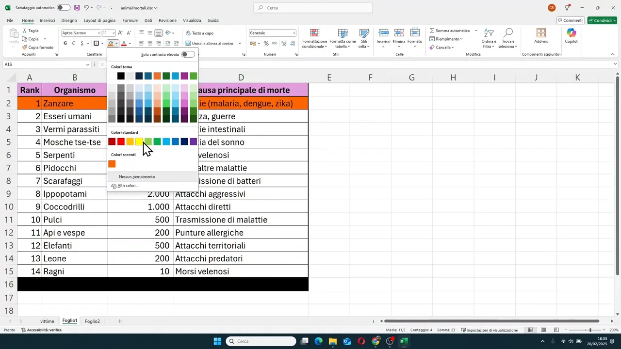
🎨 Coloring headers, the first row, and the last row

After arranging the structure and numbers, we move on to the final visual touch.

In the model shown, three areas are highlighted:

• the header row with a warm color
• the first row of data with a red hue
• the last row of the table with a green hue

To do this, simply select the desired range and use the Fill Color bucket. If the standard colors aren't satisfying, you can open the advanced color palette and define a more suitable shade.

This does not only serve to make the table look better. It also helps guide the reading. The header becomes immediately recognizable, while the first and last rows take on a special significance.

📝 Renaming the sheet to avoid confusion

We often work well inside the table, but forget a fundamental detail: the name of the sheet.

Leaving a generic name like Sheet1 is one of the most common mistakes, especially when you start having more files.

To rename it:

1. go to the sheet tab at the bottom
2. double-click on the current name
3. type a clearer and more descriptive name

In the example, a name related to the table's content is assigned. It is a small detail, but it helps a lot when you need to find your work later.

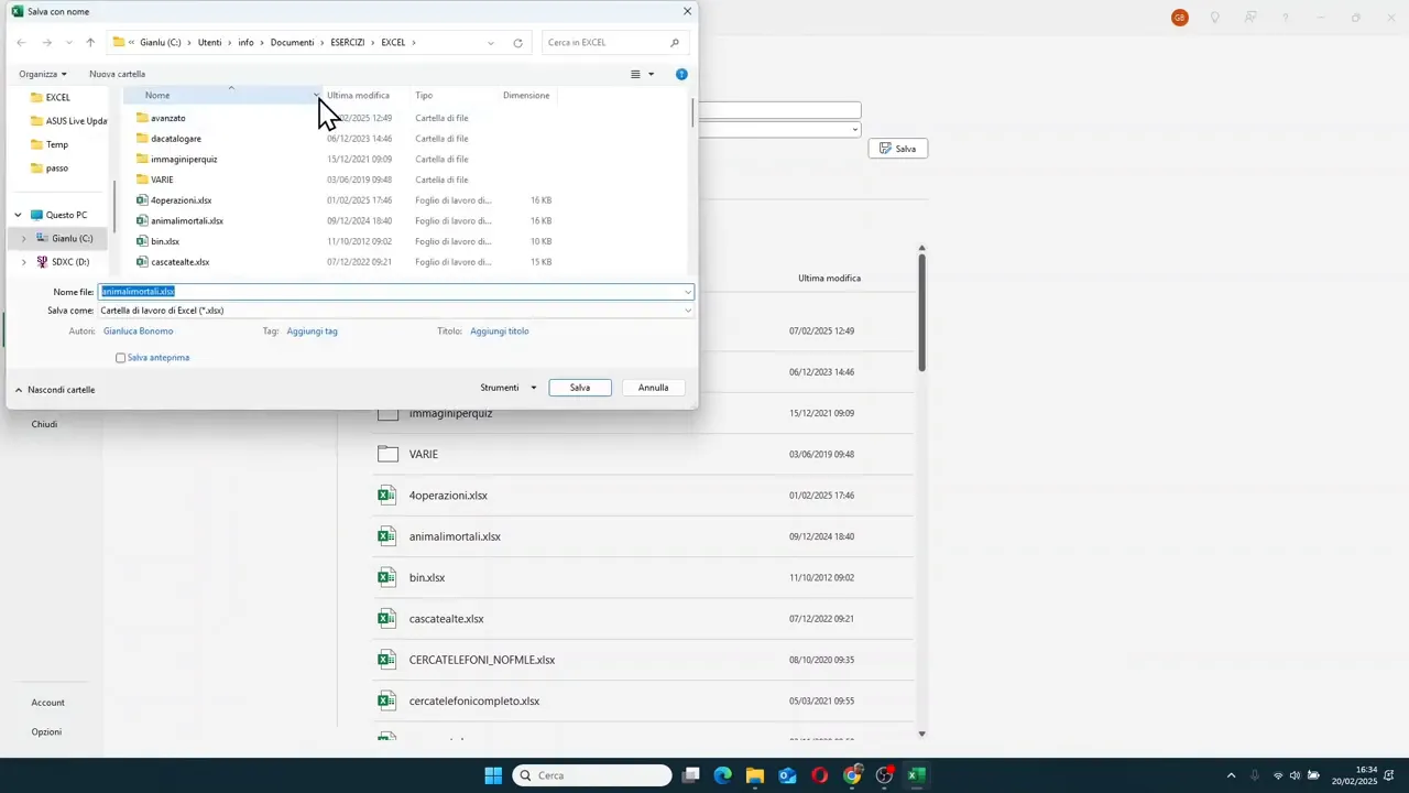
💾 Saving the file the right way

Last but decisive step: saving the file with criteria.

It is not enough to just click Save. You also need to choose:

• the folder where you want to place the file
• a clear name that allows you to recognize it immediately

If you start from a new file, Excel will ask you where to save it and what to call it. It is better to use a sensible name, not a random one, otherwise after a few days you might not remember what it contains.

In practice:

1. go to File
2. choose Save or Save As
3. use Browse to find the correct folder
4. type the file name
5. confirm with Save

✅ The final result

In the end, you have a complete, organized, and readable table, built entirely from scratch. And above all, you have put together some basic skills that are constantly needed in Excel:

• entering data correctly
• adjusting column width
• aligning and enhancing text
• formatting numbers
• applying borders
• using colors wisely
• renaming sheets and saving the file properly

These are simple operations, but they are the ones that really make the difference between an improvised sheet and a table presentable in a report or a presentation.

❓ FAQ